Stochastic Variational Inference (SVI) with Pyro

Published on Sunday, 24 September 2023

This is an in-depth explanation of the tutorial available at the Pyro Library Website, who have adapted it from Chapter 7 of the excellent book Statistical Rethinking by Richard McElreath. It refers to the work of the paper Ruggedness: The blessing of bad geography in Africa. The goal of this exercise is to explore the relationship between topographic heterogeneity of a nation as measured by the Terrain Ruggedness Index and its GDP per capita.

Abstract of Ruggedness: The blessing of bad geography in Africa

We show that geography, through its impact on history, can have important effects on current economic development. The analysis focuses on the historic interaction between ruggedness and Africa’s slave trades. Although rugged terrain hinders trade and most productive activities, negatively affecting income globally, within Africa rugged terrain afforded protection to those being raided during the slave trades. Since the slave trades retarded subsequent economic development, within Africa ruggedness has also had a historic indirect positive effect on income. Studying all countries worldwide, we estimate the differential effect of ruggedness on income for Africa. We show that:

the differential effect of ruggedness is statistically significant and economically meaningful,
it is found in Africa only,
it cannot be explained by other factors like Africa’s unique geographic environment, and
it is fully accounted for by the history of the slave trades.

We model the analysis of these data points in Pyro as given below.

Set Up

Importing the Required Libraries

%reset -s -f

import logging
import os

import torch
import numpy as np
import pandas as pd
import seaborn as sns
import matplotlib.pyplot as plt

import pyro

smoke_test = ('CI' in os.environ)
assert pyro.__version__.startswith('1.8.6')

pyro.enable_validation(True)
pyro.set_rng_seed(1)
logging.basicConfig(format='%(message)s', level=logging.INFO)

# Set matplotlib settings
%matplotlib inline
plt.style.use('default')

import pyro.distributions as dist
import pyro.distributions.constraints as constraints

Importing the data

# Importing Data
DATA_URL = "https://d2hg8soec8ck9v.cloudfront.net/datasets/rugged_data.csv"
data = pd.read_csv(DATA_URL, encoding="ISO-8859-1")
df = data[["cont_africa", "rugged", "rgdppc_2000"]]
df = df[np.isfinite(df.rgdppc_2000)]

# Now we log-normalize the GDP
df["rgdppc_2000"] = np.log(df["rgdppc_2000"])

# We then convert the Numpy array behind this dataframe to a
# torch.Tensor for analysis with PyTorch and Pyro.
train = torch.tensor(df.values, dtype=torch.float)
is_cont_africa, ruggedness, log_gdp = train[:, 0], train[:, 1], train[:, 2]

Note that as the variable GDP is highly skewed, we log-transform it before proceeding.

Preliminary Visualisation

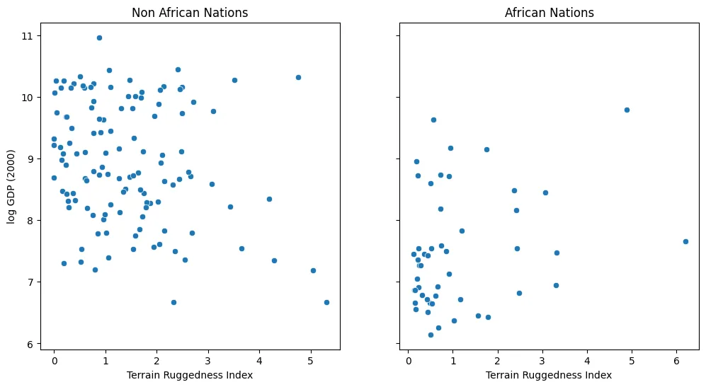
# Plot Scatter Plots
fig, ax = plt.subplots(nrows=1, ncols=2, figsize=(12, 6), sharey='all')
african_nations = df[df["cont_africa"] == 1]
non_african_nations = df[df["cont_africa"] == 0]
sns.scatterplot(x=non_african_nations["rugged"],
                y=non_african_nations["rgdppc_2000"],
                ax=ax[0])
ax[0].set(xlabel="Terrain Ruggedness Index",
          ylabel="log GDP (2000)",
          title="Non African Nations")
sns.scatterplot(x=african_nations["rugged"],
                y=african_nations["rgdppc_2000"],
                ax=ax[1])
ax[1].set(xlabel="Terrain Ruggedness Index",
          ylabel="log GDP (2000)",
          title="African Nations");

This displays a somewhat superficial claim that there is indeed a possible relationship between ruggedness and GDP, but that further analysis will be needed to confirm it.

Our Mathematical Model

We will now be implementing a Bayesian Regression Model.

Our initial hypothesis is that ruggedness has an effect on current income that is the same for all parts of the world. This relationship can be written

\begin{equation} y_i =κ_1 -\alpha r_i +βq_i +e_i \end{equation}

$i$ indexes countries
$y_i$ is income per capita,
$r_i$ is our measure of ruggedness,
$q_i$ is a measure of the efficiency or quality of the organisation of society,
$κ_1$ , $\alpha$ and $β$ are constants ( $\alpha > 0$ and $β > 0$ ),
and $e_i$ is a classical error term (i.e., we assume that the $e_i$ ‘s are independent and identically distributed, following a normal distribution with an expectation of zero).

In equation $(1)$ , we assume that the common impact of ruggedness on income is negative. This is not important for the exposition. It simply anticipates our empirical findings of a negative common effect of ruggedness.

Historical studies and the empirical work of Nunn (2008) have documented that Africa’s slave trades adversely affected the political and social structures of societies. We capture this effect of Africa’s slave trades with the following equation

\begin{equation} \begin{align*} q_i =\quad & κ_2 -\gamma x_i +u_i \quad \text{if i is in Africa}, \\ &u_i \quad \text{otherwise} \end{align*} \end{equation}

where $x_i$ denotes slave exports, $κ_2$ and $\gamma$ are constants $(\gamma > 0)$ , and $u_i$ is a classical error term.

Historical accounts argue that the number of slaves taken from an area was reduced by the ruggedness of the terrain. This relationship is given by

\begin{equation} x_i = κ_3 - λr_i + v_i \end{equation}

where $κ_3$ and $λ$ are constants $(λ > 0)$ , and $v_i$ is a classical error term.

Equations $(1)$ , $(2)$ and $(3)$ are essential relationships in our analysis. We combine all three into one and rename variables to get the fundamental relationship for our model.

\begin{align*} y &= β_0 + r_i (β_1 + β_2 I_i^{Africa}) + β_3 I_i^{Africa} + ε\\ y &= β_0 + r_i \gamma + β_3 I_i^{Africa} + ε \end{align*}

where $I^{Africa}$ is an indicator variable that equals $1$ if $i$ is in Africa and $0$ otherwise, $r_i$ is our measure of ruggedness, $\beta_0$ , $\gamma$ , $\beta_3$ are constants, and $\epsilon$ is a classical error term.

def model(is_cont_africa, ruggedness, log_gdp=None):
    a = pyro.sample("a", dist.Normal(0., 10.))
    b_s = pyro.sample("bS", dist.Normal(0., 1.))
    b_r = pyro.sample("bR", dist.Normal(0., 1.))
    b_sr = pyro.sample("bSR", dist.Normal(0., 1.))
    sigma = pyro.sample("sigma", dist.Uniform(0., 10.))

    mean = a + b_r * ruggedness + is_cont_africa * (b_s + b_sr * ruggedness)

    with pyro.plate("data", len(ruggedness)):
        return pyro.sample("obs", dist.Normal(mean, sigma), obs=log_gdp)

In a Bayesian Linear Regression model, we need to specify prior distributions on the parameters $\alpha \in\mathbb R$ (represented by a) and $\beta \in\mathbb R^3$ (expanded here into scalars b_a, b_r, and b_ar). These are probability distributions that represent our beliefs prior to observing any data about reasonable values for $\alpha$ and $\beta$ . We will also add a random scale parameter $\sigma$ that controls the observation noise.

For the constant term $\alpha$ , we use a Normal prior with a large standard deviation to indicate our relative lack of prior knowledge about baseline GDP.
For the other regression coefficients, we use standard Normal priors (centered at 0) to represent our lack of apriori knowledge of whether the relationship between covariates and GDP is positive or negative.
For the observation noise $\sigma$ , we use a flat prior bounded below by $0$ because this value must be positive to be a valid standard deviation.

Process of Inference

Notation Through out the mathematical references in this document, these notations will remain consistent:

$\textbf x \in \mathbb R^n (n \geq 1)$ - The vector of observed variables. For us, the observed variables are rugged, is_cont_africa, rgdppc_2000
$\textbf z \in \mathbb R^n (n \geq 1)$ - The vector of latent variables. For us, the latent variables are a, b_r, b_s, b_sr, sigma
$\theta \in \mathbb R^n (n \geq 1)$ - The vector of learnable parameters. As the latent variables are represented by probability distributions, the learnable parameters are the parameters of these probability distributions.

Now that we have specified a model, Bayes’ rule tells us how to use it to perform inference, or draw conclusions about latent variables from data: compute the posterior distribution over $\textbf{z}$ :

p_\theta(\textbf{z} \mid \textbf{x}) = \frac{p_\theta(\textbf{x}, \textbf{z})}{\int d\textbf{z} \quad p_\theta(\textbf{x}, \textbf{z})}

To check the results of modeling and inference, we would like to know how well a model fits observed data $\textbf x$ , which we can quantify with the evidence or marginal likelihood

p_\theta(\textbf{x}) = \int d\textbf{z} \quad p_\theta(\textbf{x}, \textbf{z})

and also to make predictions for new data, which we can do with the posterior predictive distribution

p_\theta(x' \mid \textbf{x}) = \int d\textbf{z} \quad p_\theta(x' \mid \textbf{z}) p_\theta(\textbf{z} \mid \textbf{x})

We aim to learn the parameters $\theta$ of our models from observed data $\textbf{x}$ , by maximising the marginal likelihood:

\theta_{max} = \argmax_{\theta} p_\theta(\textbf{x})

Estimating the Learnable Parameters

Guide

Each of these computations (the posterior distribution, the marginal likelihood and the posterior predictive distribution) requires performing integrals that are often impossible or computationally intractable.

While Pyro includes support for many different exact and approximate inference algorithms, the best-supported is variational inference, which offers a unified scheme for finding $\theta_{max}$ and computing a tractable approximation $q_\phi(\textbf{z})$ to the true, unknown posterior $p_{\theta_{max}}(\textbf z \mid \textbf x)$ by converting the intractable integrals into optimization of a functional of $p$ and $q$ .

This distribution $q_\phi$ is called the variational distribution in much of the literature, and in the context of Pyro it’s called the guide.

Just like the model, the guide is encoded as a Python program guide() that contains pyro.sampleand pyro.param statements. It does not contain observed data, since the guide needs to be a properly normalised distribution so that it is easy to sample from.

Note: We have implemented a guide that assumes that there is no correlation amongst the latent variables. (AutoNormal)

def custom_guide(is_cont_africa, ruggedness, log_gdp=None):
    a_loc = pyro.param('a_loc', lambda: torch.tensor(0.))
    a_scale = pyro.param('a_scale', lambda: torch.tensor(1.),
                         constraint=constraints.positive)
    sigma_loc = pyro.param('sigma_loc', lambda: torch.tensor(1.),
                             constraint=constraints.positive)
    weights_loc = pyro.param('weights_loc', lambda: torch.randn(3))
    weights_scale = pyro.param('weights_scale', lambda: torch.ones(3),
                               constraint=constraints.positive)
    a = pyro.sample("a", dist.Normal(a_loc, a_scale))
    b_s = pyro.sample("bS", dist.Normal(weights_loc[0], weights_scale[0]))
    b_r = pyro.sample("bR", dist.Normal(weights_loc[1], weights_scale[1]))
    b_sr = pyro.sample("bSR", dist.Normal(weights_loc[2], weights_scale[2]))
    sigma = pyro.sample("sigma", dist.Normal(sigma_loc, torch.tensor(0.05)))
    return {"a": a, "b_s": b_s, "b_r": b_r, "b_sr": b_sr, "sigma": sigma}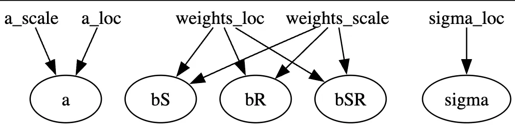

We can achieve this result by simply using:

auto_guide = pyro.infer.autoguide.AutoNormal(model)
pyro.render_model(auto_guide,
                  model_args=(is_cont_africa, ruggedness, log_gdp),
                  render_params=True)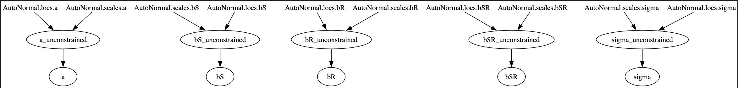

ELBO Minimisation

Variational inference approximates the true posterior by searching the space of variational distributions to find one that is most similar to the true posterior according to some measure of distance or divergence (Kullback-Leibler divergence $KL(q_\phi(\textbf{z})|| p_{\theta_{max}}(\textbf z \mid \textbf x))$ ), but computing this directly requires knowing the true posterior ahead of time, which would defeat the purpose.

We are interested in optimising this divergence, which might sound even harder, but in fact it is possible to use Bayes’ theorem to rewrite the definition of $KL(q_\phi(\textbf{z})|| p_{\theta_{max}}(\textbf z \mid \textbf x))$ as the difference between an intractable constant that does not depend on $q_\phi$ and a tractable term called the evidence lower bound (ELBO), defined below. Maximising this tractable term will therefore produce the same solution as minimising the original $KL$ -divergence.

%%time
pyro.clear_param_store()

# These should be reset each training loop.
auto_guide = pyro.infer.autoguide.AutoNormal(model)
adam = pyro.optim.Adam({"lr": 0.02})  # Consider decreasing learning rate.
elbo = pyro.infer.Trace_ELBO()
svi = pyro.infer.SVI(model, auto_guide, adam, elbo)

losses = []
for step in range(1000 if not smoke_test else 2):  # Consider running for more steps.
    loss = svi.step(is_cont_africa, ruggedness, log_gdp)
    losses.append(loss)
    if step % 100 == 0:
        logging.info("Elbo loss: {}".format(loss))

plt.figure(figsize=(5, 2))
plt.plot(losses)
plt.xlabel("SVI step")
plt.ylabel("ELBO loss");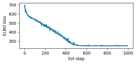

At the end of this code block, we print the values of the learnable parameters which are stored in the param_store

for name, value in pyro.get_param_store().items():
    print(name, pyro.param(name).data.cpu().numpy())

AutoNormal.locs.a 9.176606
AutoNormal.scales.a 0.07974657
AutoNormal.locs.bS -1.8880633
AutoNormal.scales.bS 0.13369536
AutoNormal.locs.bR -0.18150033
AutoNormal.scales.bR 0.042435974
AutoNormal.locs.bSR 0.3381295
AutoNormal.scales.bSR 0.08354119
AutoNormal.locs.sigma -2.2117462
AutoNormal.scales.sigma 0.053564996

By plotting a histogram of the density(frequency) of slope of the $\log$ (GDP) vs. Terrain Ruggedness graph, i.e. the slope of the regression line ( $\gamma$ ), we reiterate on the fact that $\gamma$ approximately follows a normal distribution.

with pyro.plate("samples", 800, dim=-1):
    samples = auto_guide(is_cont_africa, ruggedness)

gamma_within_africa = samples["bR"] + samples["bSR"]
gamma_outside_africa = samples["bR"]

fig = plt.figure(figsize=(10, 6))
sns.histplot(gamma_within_africa.detach().cpu().numpy(),
             kde=True, stat="density",
             label="African nations")
sns.histplot(gamma_outside_africa.detach().cpu().numpy(),
             kde=True, stat="density",
             label="Non-African nations",
             color="orange")
fig.suptitle("Density of Slope : log(GDP) vs. Terrain Ruggedness")
plt.xlabel("Slope of regression line")
plt.legend()
plt.show()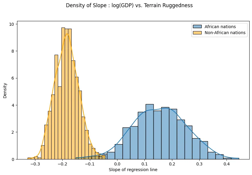

Making Predictions with the Learned Model

We now calculate the posterior predictive distribution for this model, with the guide as auto_guide, and pick out $800$ samples from it. Next we use this to determine the $90\%$ confidence interval for our data.

predictive = pyro.infer.Predictive(model,guide=auto_guide, num_samples=800)
svi_samples = predictive(is_cont_africa, ruggedness, log_gdp=None)
svi_gdp = svi_samples["obs"]

predictions = pd.DataFrame({
    "cont_africa": is_cont_africa,
    "rugged": ruggedness,
    "y_mean": svi_gdp.mean(0).detach().cpu().numpy(),
    "y_perc_5": svi_gdp.kthvalue(int(len(svi_gdp) * 0.05), dim=0)[0].detach().cpu().numpy(),
    "y_perc_95": svi_gdp.kthvalue(int(len(svi_gdp) * 0.95), dim=0)[0].detach().cpu().numpy(),
    "true_gdp": log_gdp,
})
african_nations = predictions[predictions["cont_africa"] == 1].sort_values(by=["rugged"])
non_african_nations = predictions[predictions["cont_africa"] == 0].sort_values(by=["rugged"])

fig, ax = plt.subplots(nrows=1, ncols=2, figsize=(12, 6), sharey='all')
fig.suptitle("Posterior predictive distribution with 90% CI", fontsize=16)

ax[0].plot(non_african_nations["rugged"], non_african_nations["y_mean"])
ax[0].fill_between(non_african_nations["rugged"],
                   non_african_nations["y_perc_5"],
                   non_african_nations["y_perc_95"], alpha=0.5)
ax[0].plot(non_african_nations["rugged"], non_african_nations["true_gdp"], "o")
ax[0].set(xlabel="Terrain Ruggedness Index", ylabel="log GDP (2000)", title="Non African Nations")

ax[1].plot(african_nations["rugged"], african_nations["y_mean"])
ax[1].fill_between(african_nations["rugged"],
                   african_nations["y_perc_5"],
                   african_nations["y_perc_95"], alpha=0.5)
ax[1].plot(african_nations["rugged"], african_nations["true_gdp"], "o")
ax[1].set(xlabel="Terrain Ruggedness Index", ylabel="log GDP (2000)", title="African Nations");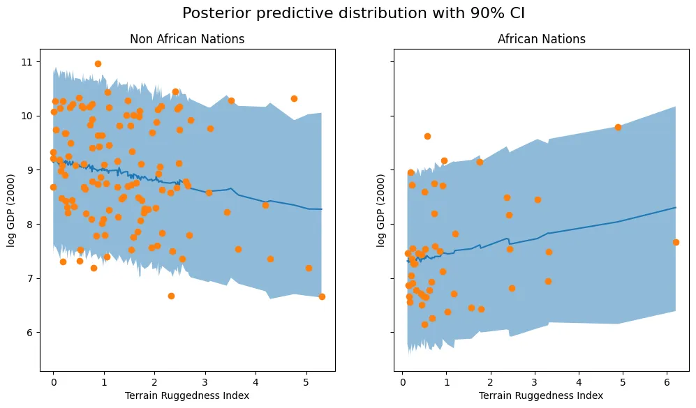

Appendix: Models in Pyro

Probabilistic models in Pyro are specified as Python functions model(*args, **kwargs) that generate observed data from latent variables using special primitive functions whose behaviour can be changed by Pyro’s internals depending on the high-level computation being performed.

Specifically, the different mathematical pieces of model() are encoded via the mapping:

latent random variables $\iff$ pyro.sample
observed random variables $\iff$ pyro.sample with the obs keyword argument
learnable parameters $\iff$ pyro.param
plates $\iff$ pyro.plate context managers

The `pyro.sample` Primitive

Probabilistic programs in Pyro are built up around samples from primitive probability distributions, marked by pyro.sample:

def sample(
    name: str,
    fn: pyro.distributions.Distribution,
    *,
    obs: typing.Optional[torch.Tensor] = **None**,
    infer: typing.Optional[dict] = **None**) -> torch.Tensor:
    ...

obs = pyro.sample("obs", dist.Normal(mean, sigma), obs=log_gdp)

However, note that when any sample statement is observed, the cumulative effect of every other sample statement in a model changes following Bayes’ rule; it is the job of Pyro’s inference algorithms to “run the program backwards” and assign mathematically consistent values to all pyro.samplestatements in a model.

The `pyro.param` Primitive

The next primitive used in our model, pyro.param, is a frontend for reading from and writing to Pyro’s key-value parameter store:

def param(
    name: str,
    init: Optional[Union[torch.Tensor, Callable[..., torch.Tensor]]] = **None**,
    *,
    constraint: torch.distributions.constraints.Constraint = constraints.real
) -> torch.Tensor:
    ...

Like pyro.sample, pyro.param is always called with a name as its first argument. The first time pyro.param is called with a particular name, it stores the initial value specified by the second argument init in the parameter store and then returns that value. After that, when it is called with that name, it returns the value from the parameter store regardless of any other arguments. After a parameter has been initialised, it is no longer necessary to specify init to retrieve its value (e.g. pyro.param("a")).
The second argument, init, can be either a torch.Tensor or a function that takes no arguments and returns a tensor. The second form is useful because it avoids repeatedly constructing initial values that are only used the first time a model is run.
The optional third argument to pyro.param, constraint, is a torch.distributions.constraints.Constraint object stored when a parameter is initialised; constraints are reapplied after every update. Pyro ships with a large number of predefined constraints.

pyro.param values persist across model calls, unless the parameter store is updated by an optimization algorithm or cleared via pyro.clear_param_store(). Unlike pyro.sample, pyro.param can be called with the same name multiple times in a model; every call with the same name will return the same value. The global parameter store itself is accessible by calling pyro.get_param_store().

The `pyro.plate` Primitive

pyro.plate is Pyro’s formal encoding of plate notation, widely used in probabilistic machine learning to simplify visualisation and analysis of models with lots of conditionally independent and identically distributed random variables.

def plate(
    name: str,
    size: int,
    *,
    dim: Optional[int] = **None**,
    **other_kwargs
) -> contextlib.AbstractContextManager:
    ...

Table of Contents